Finding the Mode of an Empirical Continuous Distribution

Let’s say you have some function f that generates samples from an unknown continuous probability distribution:

def f(n: int) -> np.ndarray:
    """Generate n samples from an unknown distribution"""
    samples = # ??? We don't know ???
    return samples

The sample generating logic could be literally unknown (as above), or it could be some complex thing that we do know but can’t easily model with a parameterized distribution. You still might want to know the mode.

How do you estimate the mode of this distribution?

In case you’re thinking “that’s obvious”, let me run through a couple solutions that don’t work.

You can’t count occurrences of values found in samples. That would work for a discrete distribution with a known set of possible values. But you can’t expect to find more than one occurrence of any of the values in samples. Mathematically, you will never get the same value twice. On a computer you will eventually get some samples twice because of finite precision, but that won’t be a good estimate of the mode of the distribution.
You can’t estimate it with the mean or median. The distribution might not be symmetric! And it might be multi-modal! If you can reasonably fit a named distribution to your samples, then the problem becomes easier: estimate the distribution parameters and look up the mode online!

Ok, so the solution isn’t obvious (at least it wasn’t obvious to me), but that doesn’t mean it’s complex. If you can generate (or already have) samples, you should start by plotting the distribution with a histogram.

Let’s write an f function so we can take a look:

import numpy as np
import pandas as pd

def f(n: int) -> np.ndarray:
    """Generate n samples from an unknown distribution"""
    df = pd.read_csv("https://jbencook.s3.amazonaws.com/data/dummy-sales-large.csv")
    np.random.seed(1)
    samples = np.random.choice(df.revenue, n)
    return samples

Now plot the distribution:

import seaborn as sns

sns.histplot(f(1000), bins=20);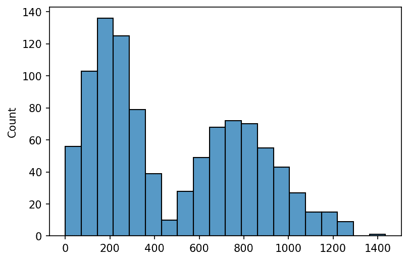

Just by looking at the plot, we can tell that the mode of this distribution is slightly less than 200. So how do you find the mode of an empirical distribution? Well, one good method is visual inspection! Just plot the histogram and take a look.

A programmatic solution

Ok, but what if you need to find the mode programmatically? This can be accomplished with the np.histogram() function from NumPy:

counts, bins = np.histogram(x, bins=20)
max_bin = np.argmax(counts)
bins[max_bin:max_bin+2].mean()

# Expected result
# 179.3633778773795

As expected: slightly less than 200! The np.histogram() function returns two arrays, one with the number of instances per bin and one with the edges of the bins. That means we can estimate the location of the maximum height of the distribution by getting the index of the maximum count and then taking the midpoint of that bin.

Precision of the estimate

The big factor in determining how precise your estimate will be is your bin size, which you can think of as a hyperparameter for this procedure. I don’t have a great rule of thumb for picking this. What I do is plot the histogram and mess with number of bins until I achieve a “reasonable amount of smoothness”. But generally speaking, the more data you have, the more bins you can use and the more precise your estimate will be.

Why would you want the mode of a weird distribution like this?

The mode is sometimes a good pick for a “typical” value to summarize a distribution. Remember the mean is susceptible to outliers and the median will tend to have low probability density if the distribution is multi-modal. In the example we’re using the mean is around 482 and the median is around 359. Both of these are actually relatively low probability values so it might be important to estimate the mode!