Overview

This post is going to showcase the development of a vehicle speed detector using Sparrow Computing’s open-source libraries and PyTorch Lightning.

The exciting news here is that we could make this speed detector for any traffic feed without prior knowledge about the site (no calibration required), or specialized imaging equipment (no depth sensors required). Better yet, we only needed ~300 annotated images to reach a decent speed estimate. To estimate speed, we will detect all vehicles coming toward the camera using an object detection model. We will also predict the locations of the back tire and the front tire of every vehicle using a keypoint model. Finally, we will perform object tracking to account for the same tire as it progresses frame-to-frame so that we can estimate vehicle speed.

Without further ado, let’s dive in…

What we will need

• A video stream of automobile traffic
• About 300 randomly sampled video frames from the video stream
• Bounding box annotations around all the vehicles moving toward the camera
• Keypoint annotations for the points where the front tire and the back tire touch the road (on the side where the vehicle is facing the camera)

End-to-end Pipeline

The computer vision system we are building takes in a traffic video as an input, makes inferences through multiple deep learning models, and generates 1) an annotated video and 2) a traffic log that prints vehicle counts and speeds. The figure below is a high-level overview of how the whole system is glued together (numbered in chronological order). We will talk about each of the nine process units as well as the I/O highlighted in green.

Docker Container Setup

First, we need a template that comes with the dependencies and configuration for Sparrow’s development environment. This template can be generated with a Python package called sparrow-patterns. After creating the project source directory, the project will run in a Docker container so that our development will be platform-independent.

To set this up, all you have to do is:

pip install sparrow-patterns
sparrow-patterns project speed-trapv3

Before you run the template on a container, add an empty file called .env inside the folder named .devcontainer as shown below.

Input Annotation Files

For this project, we used an annotation platform called V7 Darwin, but the same approach would work with other annotation platforms.

The Darwin annotation file (shown below) is a JSON object for each image that we tag. Note that “id” is a hash value that uniquely identifies an object on the frame that is only relevant to the Darwin platform. The data we need is contained in the “bounding_box” and “name” objects. Once you have annotations, you need to convert them to a form that PyTorch’s Dataset class is looking for:

{
  "annotations": [
    {
      "bounding_box": {
        "h": 91.61,
        "w": 151.53,
        "x": 503.02,
        "y": 344.16
      },
      "id": "ce9d224b-0963-4a16-ba1c-34a2fc062b1b",
      "name": "vehicle"
    },
    {
      "id": "8120d748-5670-4ece-bc01-6226b380e293",
      "keypoint": {
        "x": 508.47,
        "y": 427.1
      },
      "name": "back_tire"
    },
    {
      "id": "3f71b63d-d293-4862-be7b-fa35b76b802f",
      "keypoint": {
        "x": 537.3,
        "y": 434.54
      },
      "name": "front_tire"
    }
  ],
  }

Object Detection Model

Define the dataset

In the Dataset class, we create a dictionary with keys such as the frame of the video, the bounding boxes of the frame, and the labels for each of the bounding boxes. The values of that dictionary are then stored as PyTorch tensors. The following is the generic setup for the Dataset class:

class RetinaNetDataset(torch.utils.data.Dataset):  # type: ignore
    """Dataset class for RetinaNet model."""

    def __init__(self, holdout: Optional[Holdout] = None) -> None:
        self.samples = get_sample_dicts(holdout)
        self.transform = T.ToTensor()

    def __len__(self) -> int:
        """Return number of samples."""
        return len(self.samples)

    def __getitem__(self, idx: int) -> dict[str, torch.Tensor]:
        """Get the tensor dict for a sample."""
        sample = self.samples[idx]
        img = Image.open(sample["image_path"])
        x = self.transform(img)
        boxes = sample["boxes"].astype("float32")
        return {
            "image": x,
            "boxes": torch.from_numpy(boxes),
            "labels": torch.from_numpy(sample["labels"]),
        }

Define the model

We use a pre-trained RetinaNet model from TorchVision as our detection model defined in the Module class:

from torchvision import models


class RetinaNet(torch.nn.Module):
    """Retinanet model based on Torchvision"""

    def __init__(
        self,
        n_classes: int = Config.n_classes,
        min_size: int = Config.min_size,
        trainable_backbone_layers: int = Config.trainable_backbone_layers,
        pretrained: bool = False,
        pretrained_backbone: bool = True,
    ) -> None:
        super().__init__()
        self.n_classes = n_classes
        self.model = models.detection.retinanet_resnet50_fpn(
            progress=True,
            pretrained=pretrained,
            num_classes=n_classes,
            min_size=min_size,
            trainable_backbone_layers=trainable_backbone_layers,
            pretrained_backbone=pretrained_backbone,
        )

Notice that the forward method (below) of the Module class returns the bounding boxes, confidence scores for the boxes, and the assigned labels for each box in form of tensors stored in a dictionary.

def forward(
        self,
        x: Union[npt.NDArray[np.float64], list[torch.Tensor]],
        y: Optional[list[dict[str, torch.Tensor]]] = None,
    ) -> Union[
        dict[str, torch.Tensor], list[dict[str, torch.Tensor]], FrameAugmentedBoxes
    ]:
        """
        Forward pass for training and inference.

        Parameters
        ----------
        x
            A list of image tensors with shape (3, n_rows, n_cols) with
            unnormalized values in [0, 1].
        y
            An optional list of targets with an x1, x2, y1, y2 "boxes" tensor
            and a class index "labels" tensor.

        Returns
        -------
        result(s)
            If inference, this will be a list of dicts with predicted tensors
            for "boxes", "scores" and "labels" in each one. If training, this
            will be a dict with loss tensors for "classification" and
            "bbox_regression".
        """
        if isinstance(x, np.ndarray):
            return self.forward_numpy(x)
        elif self.training:
            return self.model.forward(x, y)
        results = self.model.forward(x, y)
        padded_results = []
        for result in results:
            padded_result: dict[str, torch.Tensor] = {}
            padded_result["boxes"] = torch.nn.functional.pad(
                result["boxes"], (0, 0, 0, Config.max_boxes), value=-1.0
            )[: Config.max_boxes]
            padded_result["scores"] = torch.nn.functional.pad(
                result["scores"], (0, Config.max_boxes), value=-1.0
            )[: Config.max_boxes]
            padded_result["labels"] = torch.nn.functional.pad(
                result["labels"], (0, Config.max_boxes), value=-1
            )[: Config.max_boxes].float()
            padded_results.append(padded_result)
        return padded_results

With that, we should be able to train and save the detector as a .pth file, which stores trained PyTorch weights.

One important detail to mention here is that the dictionary created during inference is converted into a Sparrow data structure called FrameAugmentedBox from the sparrow-datums package. In the following code snippet, the results_to_boxes() function converts the inference result into a FrameAugmentedBox object. We convert the inference results to Sparrow format so they can be directly used with other Sparrow packages such as sparrow-tracky which is used to perform object tracking later on.

def result_to_boxes(
    result: dict[str, torch.Tensor],
    image_width: Optional[int] = None,
    image_height: Optional[int] = None,
) -> FrameAugmentedBoxes:
    """Convert RetinaNet result dict to FrameAugmentedBoxes."""
    box_data = to_numpy(result["boxes"]).astype("float64")
    labels = to_numpy(result["labels"]).astype("float64")
    if "scores" in result:
        scores = to_numpy(result["scores"]).astype("float64")
    else:
        scores = np.ones(len(labels))
    mask = scores >= 0
    box_data = box_data[mask]
    labels = labels[mask]
    scores = scores[mask]
    return FrameAugmentedBoxes(
        np.concatenate([box_data, scores[:, None], labels[:, None]], -1),
        ptype=PType.absolute_tlbr,
        image_width=image_width,
        image_height=image_height,
    )

Now, we can use the saved detection model to make inferences and obtain the predictions as FrameAugmentedBoxes.

Object Detection Evaluation

To quantify the performance of the detection model, we use MOTA (Multiple Object Tracking Accuracy) as the primary metric, which has a range of [-inf, 1.0], where perfect object tracking is indicated by 1.0. Since we have not performed tracking yet, we will estimate MOTA without the identity switches. Just for the sake of clarity, we will call it MODA (Multiple Object Detection Accuracy). To calculate MODA, we use a method called compute_moda() from the sparrow-tracky package which employs the pairwise IoU between bounding boxes to find the similarity.

from sparrow_tracky import compute_moda

moda = 0
count = 0
for batch in iter(test_dataloader):
    x = batch['image']
    x = x.cuda()
    sample = {'boxes':batch['boxes'][0], 'labels':batch['labels'][0]}
    result = detection_model(x)[0]
    predicted_boxes = result_to_boxes(result)
    predicted_boxes = predicted_boxes[predicted_boxes.scores > DetConfig.score_threshold]
    ground_truth_boxes = result_to_boxes(sample)
    frame_moda = compute_moda(predicted_boxes, ground_truth_boxes)
    moda += frame_moda.value
    count += 1
print(f"Based on {count} test examples, the Multiple Object Detection Accuracy is {moda/count}.")

The MODA for our detection model turned out to be 0.98 based on 43 test examples, indicating that our model has high variance, so the model would not be as effective if we used a different video. To improve the high variance, we will need more training examples.

Object Tracking

Now that we have the trained detection model saved as a .pth file, we run an inference with the detection model and perform object tracking at the same time. The source video is split into video frames and detection predictions for a frame are converted into a FrameAugmentedBox as explained before. Later, it is fed into a Tracker object that is instantiated from Sparrow’s sparrow-tracky package. After looping through all the frames, the Tracker object tracks the vehicles using an algorithm similar to SORT (you can read more about our approach here). Finally, the data stored in the Tracker object is written into a file using a Sparrow data structure. The file will have an extension of .json.gz when it is saved.

from sparrow_tracky import Tracker


def track_objects(
    video_path: Union[str, Path],
    model_path: Union[str, Path] = Config.pth_model_path,
) -> None:
    """
    Track ball and the players in a video.
    Parameters
    ----------
    video_path
        The path to the source video
    output_path
        The path to write the chunk to
    model_path
        The path to the ONNX model
    """
    video_path = Path(video_path)
    slug = video_path.name.removesuffix(".mp4")
    vehicle_tracker = Tracker(Config.vehicle_iou_threshold)
    detection_model = RetinaNet().eval().cuda()
    detection_model.load(model_path)
    fps, n_frames = get_video_properties(video_path)
    reader = imageio.get_reader(video_path)
    for i in tqdm(range(n_frames)):
        data = reader.get_data(i)
        data = cv2.rectangle(
            data, (450, 200), (1280, 720), thickness=5, color=(0, 255, 0)
        )
        # input_height, input_width = data.shape[:2]
        aug_boxes = detection_model(data)
        aug_boxes = aug_boxes[aug_boxes.scores > TrackConfig.vehicle_score_threshold]
        boxes = aug_boxes.array[:, :4]
        vehicle_boxes = FrameBoxes(
            boxes,
            PType.absolute_tlbr,  # (x1, y1, x2, y2) in absolute pixel coordinates [With respect to the original image size]
            image_width=data.shape[1],
            image_height=data.shape[0],
        ).to_relative()

        vehicle_tracker.track(vehicle_boxes)
    make_path(str(Config.prediction_directory / slug))
    vehicle_chunk = vehicle_tracker.make_chunk(fps, Config.vehicle_tracklet_length)
    vehicle_chunk.to_file(
        Config.prediction_directory / slug / f"{slug}_vehicle.json.gz"
    )

Tracking Evaluation

We quantify our tracking performance using MOTA (Multi Model Tracking Accuracy) from the sparrow-tracky package. Similar to MODA, MOTA has a range of [-inf, 1.0], where 1.0 indicates the perfect tracking performance. Note that we need a sample video with tracking ground truth to perform the evaluation. Further, both the predictions and the ground truth should be transformed into an AugmentedBoxTracking object to be compatible with the compute_mota() function from the sparrow-tracky package as shown below.

from sparrow_datums import AugmentedBoxTracking, BoxTracking
from sparrow_tracky import compute_mota

test_mota = compute_mota(pred_aug_box_tracking, gt_aug_box_tracking)
print("MOTA for the test video is ", test_mota.value)

The MOTA value for our tracking algorithm turns out to be -0.94 when we evaluated it against a small sample of “ground-truth” video clips, indicating that there is plenty of room for improvement.

Keypoint Model

In order to locate each tire of a vehicle, we crop the vehicles detected by the detection model, resize them, and feed them into the keypoint model to predict the tire locations.

During cropping and resizing, the x and y coordinates of the keypoints need to be handled properly. When x and y coordinates are divided by the image width and the image height, the range of the keypoints becomes [0, 1], and we use the term “relative coordinates”. Relative coordinates tell us the location of a pixel with respect to the dimensions of the image it is located at. Similarly, when keypoints are not divided by the dimensions of the frame, we use the term “absolute coordinates”, which solely relies on the frame’s Cartesian plane to establish pixel location. Assuming the keypoints are in relative coordinates when we read them from the annotation file, we have to multiply by the original frame dimensions to get the keypoints in absolute pixel space. Since the keypoint model takes in cropped regions, we have to subtract the top-left coordinate from the keypoints to change the origin of the cropped region from (0, 0) to (x1, y1). Since we resize the cropped region, we divide the shifted keypoints by the dimensions of the cropped region and then multiply by the keypoint model input size. You can visualize this process using the flow chart below.

A known fact among neural networks is that they are good at learning surfaces rather than learning a single point. Because of that, we create two Laplacian of Gaussian surfaces where the highest energy is at the location of each keypoint. These two images are called heatmaps which are stacked up on each other before feeding into the model. To visualize the heatmaps, we can combine both heatmaps into a single heatmap and superimpose it on the corresponding vehicle as shown below.

def keypoints_to_heatmap(
    x0: int, y0: int, w: int, h: int, covariance: float = Config.covariance_2d
) -> np.ndarray:
    """Create a 2D heatmap from an x, y pixel location."""
    if x0 < 0 and y0 < 0:
        x0 = 0
        y0 = 0
    xx, yy = np.meshgrid(np.arange(w), np.arange(h))
    zz = (
        1
        / (2 * np.pi * covariance**2)
        * np.exp(
            -(
                (xx - x0) ** 2 / (2 * covariance**2)
                + (yy - y0) ** 2 / (2 * covariance**2)
            )
        )
    )
    # Normalize zz to be in [0, 1]
    zz_min = zz.min()
    zz_max = zz.max()
    zz_range = zz_max - zz_min
    if zz_range == 0:
        zz_range += 1e-8
    return (zz - zz_min) / zz_range

The important fact to notice here is that if the keypoint coordinates are negative, (0, 0) is assigned. When both tires are not visible (i.e. because of occlusion), we assign (-1, -1) for the missing tire at the Dataset class since the PyTorch collate_fn() requires fixed input shapes. At the keypoints_to_heatmap() function, the negative value is zeroed out indicating that the tire is located at the top left corner of the vehicle’s bounding box as shown below.

In real life, this is impossible, since tires are located in the bottom half of the bounding box. The model learns these patterns during the training and continues to predict the missing tire in the top left corner which makes it easier for us to filter.

The Dataset class for the keypoint model could look like this:

class SegmentationDataset(torch.utils.data.Dataset):
    """Dataset class for Segmentations model."""

    def __init__(self, holdout: Optional[Holdout] = None) -> None:
        self.samples = get_sample_dicts(holdout)

    def __len__(self):
        """Length of the sample."""
        return len(self.samples)

    def __getitem__(self, idx: int) -> dict[str, torch.Tensor]:
        """Get the tensor dict for a sample."""
        sample = self.samples[idx]
        crop_width, crop_height = Config.image_crop_size
        keypoints = process_keypoints(sample["keypoints"], sample["bounding_box"])
        heatmaps = []
        for x, y in keypoints:
            heatmaps.append(keypoints_to_heatmap(x, y, crop_width, crop_height))
        heatmaps = np.stack(heatmaps, 0)
        img = Image.open(sample["image_path"])
        img = crop_and_resize(sample["bounding_box"], img, crop_width, crop_height)
        x = image_transform(img)

        return {
            "holdout": sample["holdout"],
            "image_path": sample["image_path"],
            "annotation_path": sample["annotation_path"],
            "heatmaps": heatmaps.astype("float32"),
            "keypoints": keypoints.astype("float32"),
            "labels": sample["labels"],
            "image": x,
        }

Note that the Dataset class creates a dictionary with the following keys:

• holdout: Whether the example belongs to train, dev (validation), or test set
• image_path: Stored location of the video frame
• annotation_path: Stored location of the annotation file corresponding to the frame
• heatmaps: Transformed keypoints in the form of surfaces
• labels: Labels of the keypoints
• image: Numerical values of the frame

For the Module class of the keypoint model we use a pre-trained ResNet50 architecture with a sigmoid classification top.

A high-level implementation of the Module class would be:

from torchvision.models.segmentation import fcn_resnet50


class SegmentationModel(torch.nn.Module):
    """Model for prediction court/net keypoints."""

    def __init__(self) -> None:
        super().__init__()
        self.fcn = fcn_resnet50(
            num_classes=Config.num_classes, pretrained_backbone=True, aux_loss=False
        )

    def forward(self, x: torch.Tensor) -> torch.Tensor:
        """Run a forward pass with the model."""
        heatmaps = torch.sigmoid(self.fcn(x)["out"])
        ncols = heatmaps.shape[-1]
        flattened_keypoint_indices = torch.flatten(heatmaps, 2).argmax(-1)
        xs = (flattened_keypoint_indices % ncols).float()
        ys = torch.floor(flattened_keypoint_indices / ncols)
        keypoints = torch.stack([xs, ys], -1)
        return {"heatmaps": heatmaps, "keypoints": keypoints}

    def load(self, model_path: Union[Path, str]) -> str:
        """Load model weights."""
        weights = torch.load(model_path)
        result: str = self.load_state_dict(weights)
        return result

Now, we have everything we need to train and save the model in .pth format.

Keypoints post-processing

Recall that since we transformed the coordinates of the keypoints before feeding them into the model, the keypoint predictions are going to be in absolute space with respect to the dimensions of the resized cropped region. To project them back to the original frame dimensions we have to follow a few steps mentioned in the flowchart below.

First, we have to divide the keypoints by the dimensions of the model input size, which takes the keypoints into the relative space. Then, we have to multiply them by the dimensions of the cropped region to take them back to absolute space with respect to the cropped region of interest dimensions. Despite the keypoints being back in absolute space, the origin of its coordinate system starts at (x1, y1). So, we have to add (x1, y1) to bring the origin back to (0, 0) of the original frame’s coordinate system.

Keypoint model evaluation

We quantify the model performance using the relative error metric, which is the ratio of the magnitude of the difference between ground truth and prediction compared to the magnitude of the ground truth.

overall_rel_error = 0
count = 0
for batch in iter(test_dataloader):
    x = batch['image']
    x = x.cuda()
    result = model(x)
    relative_error = torch.norm(
        batch["keypoints"].cuda() - result["keypoints"].cuda()
    ) / torch.norm(batch["keypoints"].cuda())
    overall_rel_error += relative_error
    count += 1
print(f"The relative error of the test set is {overall_rel_error * 100}%.")

The relative error of our keypoint model turns out to be 20%, which indicates that for every ground truth with a magnitude of 100 units, there is an error of 20 units in the corresponding prediction. This model is also over-fitting to some extent, so it would probably perform poorly on a different video. However, this could be mitigated by adding more training examples.

Aggregating Multi-Model Predictions

Recall that we saved the tracking results in a .json.gz file. Now, we open that file using the sparrow-datums package, merge the keypoints predictions, and write into two JSON files called objectwise_aggregation.json and framewise_aggregation.json. The motivation behind having these two files is that it allows us to access all the predictions in one place at constant time (o(1)). More specifically, the objectwise_aggregation.json dictionary keeps the order that the objects that appeared in the video as the key and all the predictions regarding that object as the value.

Here’s a list of things objectwise_aggregation.json keeps for every object:

• Frame range the object appeared
• The bounding box of each appearance
• Object tracklet ID (Unique ID assigned for each object by the SORT algorithm)

In contrast, the framewise_aggregation.json dictionary uses the frame number as the key. All the predictions related to that frame are used as the value.

The following is the list of things we can grab from each video frame:

• All the objects that appeared in that frame
• The bounding box of the objects
• Keypoints (Transformed x, y coordinates of the tires)
• Sigmoid scores of the keypoints (we used a sigmoid function to classify between the back and front tire)
• Object ID (the order that the object appeared in the input video)
• Object tracklet ID (Unique ID assigned for each object by the SORT algorithm)

Speed Algorithm

Once we have all the primitives detected from frames and videos, we will use both frame-wise and object-wise data to estimate the speed of the vehicles based on the model predictions. The simplest form of the speed algorithm would be to measure the distance between the front tire and the back tire which is known as the wheelbase at frame n, and then determine how many frames it took for the back tire to travel the wheelbase distance from frame n. For simplicity, we assume that every vehicle has the same wheelbase, which is 2.43 meters. Further, since we do not know any information about the site or the equipment, we assume that the pixel-wise wheelbase of a vehicle remains the same. Therefore, our approach works best when the camera is located at the side of the road and pointed in the orthogonal direction to the vehicles’ moving direction (which is not the case in the demo video).

Noise Filtering

Since our keypoint model has a 20% error rate, the keypoint predictions are not perfect, so we have to filter out some of the keypoints. Here are some of the observations we did to identify common scenarios where the model under-performed.

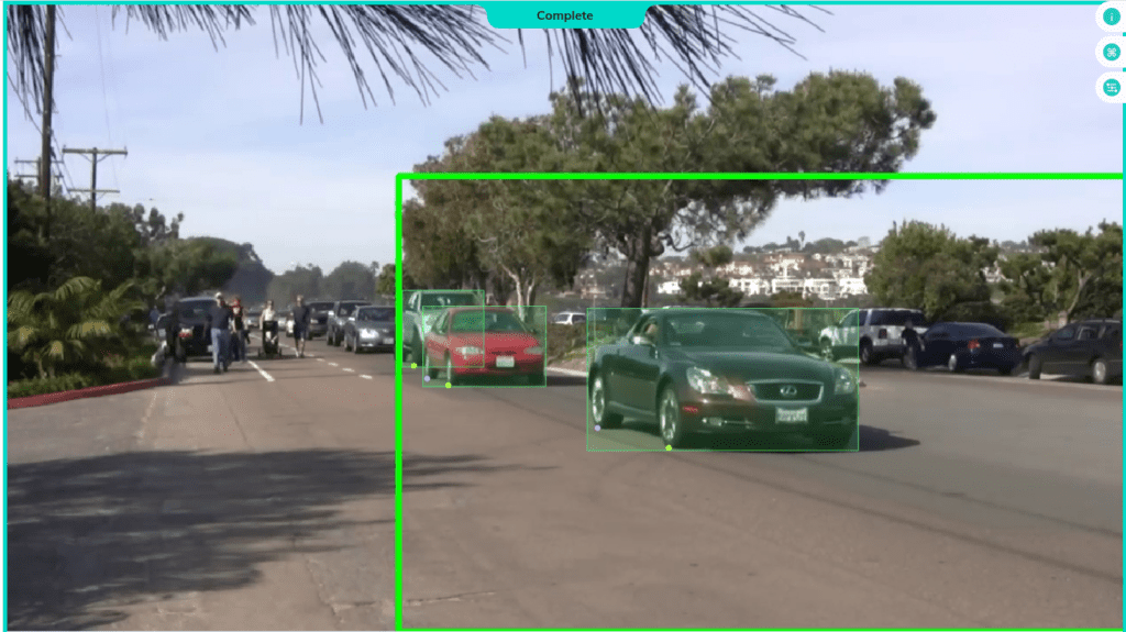
Scenario 1

Model predictions around the green boundary do not perform well since only a portion of vehicles is visible to the camera. So, it is better to wait for those vehicles to come to a better detection area. Therefore, we filter out any vehicles predictions that have x1 less than some threshold for the top-left x coordinate of their bounding box.

Scenario 2

For the missing tires, we taught the model to make predictions at the origin of the bounding box. Additionally, there are instances when the model mis-predicts the keypoint and it ends up being on the upper half of the bounding box of the vehicle. Both of these cases can be resolved by removing any keypoints that are located on the upper half of the bounding box.

Scenario 3

For missing tires, the model tends to predict both tires at the same spot, so we have to remove one of them. In this case, we could draw a circle centering the back tire and if the other tire is inside of that circle, we can get rid of the tire that had the lower probability in the sigmoid classification top.

Summary of the rules formed

So, we form three rules to filter out keypoints that are not relevant.

1. Filter out any keypoints whose top-left bounding box coordinate satisfies x1 < some threshold.
2. Ignore any keypoints that are predicted in the upper half of the bounding box.
3. Neglect the keypoint with the lower sigmoid score when tires overlap with each other.

When we plot all the keypoints predicted throughout the input video, notice that most of the tires overlap and the general trend is a straight line.

After the rules have been applied, notice that most of the outliers gets filtered out.

Also, note that some vehicles will be completely ignored leaving only four vehicles.

Filling the Missing Values

When we perform filtering, there are instances where only a single tire gets filtered out, and the other remains. To fix that, we fit keypoint data of each vehicle into a straight line using linear regression, where the x, and y coordinates of the back tire and the x coordinate of the front tire are the independent variables and the y coordinate of the front tire is the dependent variable. Using the coefficients of the fitted line, we can now predict and fill in the missing values.

For example, here’s what the straight-line trend looks like with missing values.

After predicting the missing values with linear regression, we can gain 50 more points to estimate the speed more precisely.

Speed Estimation

Now that we have complete pairs of keypoints, it’s time to jump into the geometry of the problem we are solving…

If we draw a circle around the back tire with a radius representing the pixel-wise wheelbase (d), we form the gray area defined on the diagram. Our goal is to find out which back tire that shows up in a future frame has reached the distance of d from the current back tire. Since the keypoints are still not perfect, we could land on a future back tire that is located anywhere on the circle. To remedy that, we can find the theta angle by finding alpha and beta with simple trigonometry. Then, we threshold the theta value and define that theta cannot exceed the threshold. Ideally, theta should be zero since the vehicle is traveling on a linear path. Although the future back tire and the current front tire ideally should be on the same circular boundary, there can be some errors. So, we define an upper bound (green dotted line) and a lower bound (purple dotted line) on the diagram. Let’s put this together to form an algorithm to estimate the speed.

Speed Algorithm

• Pick a pair of tires (red and yellow).
• Find the distance (d) between the chosen pair.
• From the back tire, draw a circle with a radius d.
• From that back tire, iterate through the future back tires until the distance between the current back tire and the future back tire match d.
• If d has been exceeded by more than m pixels (green boundary), ignore the current tire pair and move on to the next pair.
• If d has fallen short by more than m pixels (purple boundary), ignore the current tire pair and move on to the next pair.
• If not, find theta using alpha, beta and if theta is less than the threshold value of 𝛄, and if the number of frames from the current backfire to the future back tire is larger than 1, consider that point as eligible for speed estimation.
• Otherwise, ignore the current pair and move on to the next pair.
• Stop when all the tire pairs have been explored.
• Find out how many frames there are between the current back tire and the future back tire to find the elapsed time.
• Wheelbase (d) / elapsed time renders the instantaneous vehicle speed.

def estimate_speed(video_path_in):
    """Estimate the speed of the vehicles in the video.

    Parameters
    ----------
    video_path_in : str
        Source video path
    """
    video_path = video_path_in
    slug = Path(video_path).name.removesuffix(".mp4")
    objects_to_predictions_map = open_objects_to_predictions_map(slug)
    object_names, vehicle_indices, objectwise_keypoints = filter_bad_tire_pairs(
        video_path
    )
    speed_collection = {}
    for vehicle_index in vehicle_indices:  # Looping through all objects in the video
        approximate_speed = -1
        object_name = object_names[vehicle_index]
        coef, bias, data = straight_line_fit(objectwise_keypoints, object_name)
        (
            back_tire_x_list,
            back_tire_y_list,
            front_tire_x_list,
            front_tire_y_list,
        ) = fill_missing_keypoints(coef, bias, data)

        vehicle_speed = []
        skipped = 0

        back_tire_keypoints = [back_tire_x_list, back_tire_y_list]
        back_tire_keypoints = [list(x) for x in zip(*back_tire_keypoints[::-1])]
        front_tire_keypoints = [front_tire_x_list, front_tire_y_list]
        front_tire_keypoints = [list(x) for x in zip(*front_tire_keypoints[::-1])]

        back_tire_x_list = []
        back_tire_y_list = []
        front_tire_x_list = []
        front_tire_y_list = []
        # Speed calculation algorithm starts here...
        vehicle_speed = {}
        total_num_points = len(objectwise_keypoints[object_name])
        object_start = objects_to_predictions_map[vehicle_index]["segments"][0][0]
        for i in range(total_num_points):
            back_tire = back_tire_keypoints[i]
            front_tire = front_tire_keypoints[i]
            if back_tire[0] < 0 or front_tire[0] < 0:
                vehicle_speed[i + object_start] = approximate_speed
                skipped += 1
                continue
            for j in range(i, total_num_points):
                future_back_tire = back_tire_keypoints[j]
                if future_back_tire[0] < 0:
                    continue
                back_tire_x = back_tire[0]
                back_tire_y = back_tire[1]
                front_tire_x = front_tire[0]
                front_tire_y = front_tire[1]
                future_back_tire_x = future_back_tire[0]
                future_back_tire_y = future_back_tire[1]
                current_keypoints_distance = get_distance(
                    back_tire_x, back_tire_y, front_tire_x, front_tire_y
                )
                future_keypoints_distance = get_distance(
                    back_tire_x, back_tire_y, future_back_tire_x, future_back_tire_y
                )
                if (
                    current_keypoints_distance - future_keypoints_distance
                ) >= -SpeedConfig.distance_error_threshold and (
                    current_keypoints_distance - future_keypoints_distance
                ) <= SpeedConfig.distance_error_threshold:
                    alpha = get_angle(
                        back_tire_x, back_tire_y, future_back_tire_x, future_back_tire_y
                    )
                    beta = get_angle(
                        back_tire_x, back_tire_y, front_tire_x, front_tire_y
                    )
                    if (
                        SpeedConfig.in_between_angle >= alpha + beta
                        and (j - i) > 1
                    ):
                        approximate_speed = round(
                            SpeedConfig.MPERSTOMPH
                            * SpeedConfig.WHEEL_BASE
                            / frames_to_seconds(30, j - i)
                        )
                        vehicle_speed[i + object_start] = approximate_speed
                        back_tire_x_list.append(back_tire_x)
                        back_tire_y_list.append(back_tire_y)
                        front_tire_x_list.append(front_tire_x)
                        front_tire_y_list.append(front_tire_y)
                    break
        speed_collection[vehicle_index] = vehicle_speed
    f = open(SpeedConfig.json_directory / slug / "speed_log.json", "w")
    json.dump(speed_collection, f)
    f.close()

The instantaneous speed calculated by the algorithm is saved into a JSON file called speed_log.json which keeps track of the instantaneous speed of the detected vehicles with their corresponding frames. Also, the detected speed is printed on the video frame and all the video frames are put back together to produce the following annotated video.

After iterating through all the frames, we can use the speed log JSON file to calculate general statics such as the maximum speed, fastest vehicle, and average speed of every vehicle to create a report of the traffic in the video feed.

Conclusion

Let’s summarize what we did today. We built a computer vision system that can estimate the speed of vehicles in a given video. To estimate the speed of a vehicle, we needed to know the locations of its tires in every frame that it appeared. For that, we needed to perform three main tasks.

1. Detecting vehicles
2. Tracking the vehicles and assigning unique identities to them
3. Predicting the keypoints for every vehicle in every frame

After acquiring keypoint locations for every vehicle, we developed a geometric rule-based algorithm to estimate the number of frames it takes for the back tire of a vehicle to reach the position of its corresponding front tire’s position in the future. With that information in hand, we can approximate the speed of that vehicle.

Before we wind up our project, you can check out the complete implementation of the code here. This code would have been more complex if it wasn’t for Sparrow packages. So, make sure to check them out as well. You can find me via LinkedIn if you have any questions.